Excel Power User Functions That Still Matter in 2026

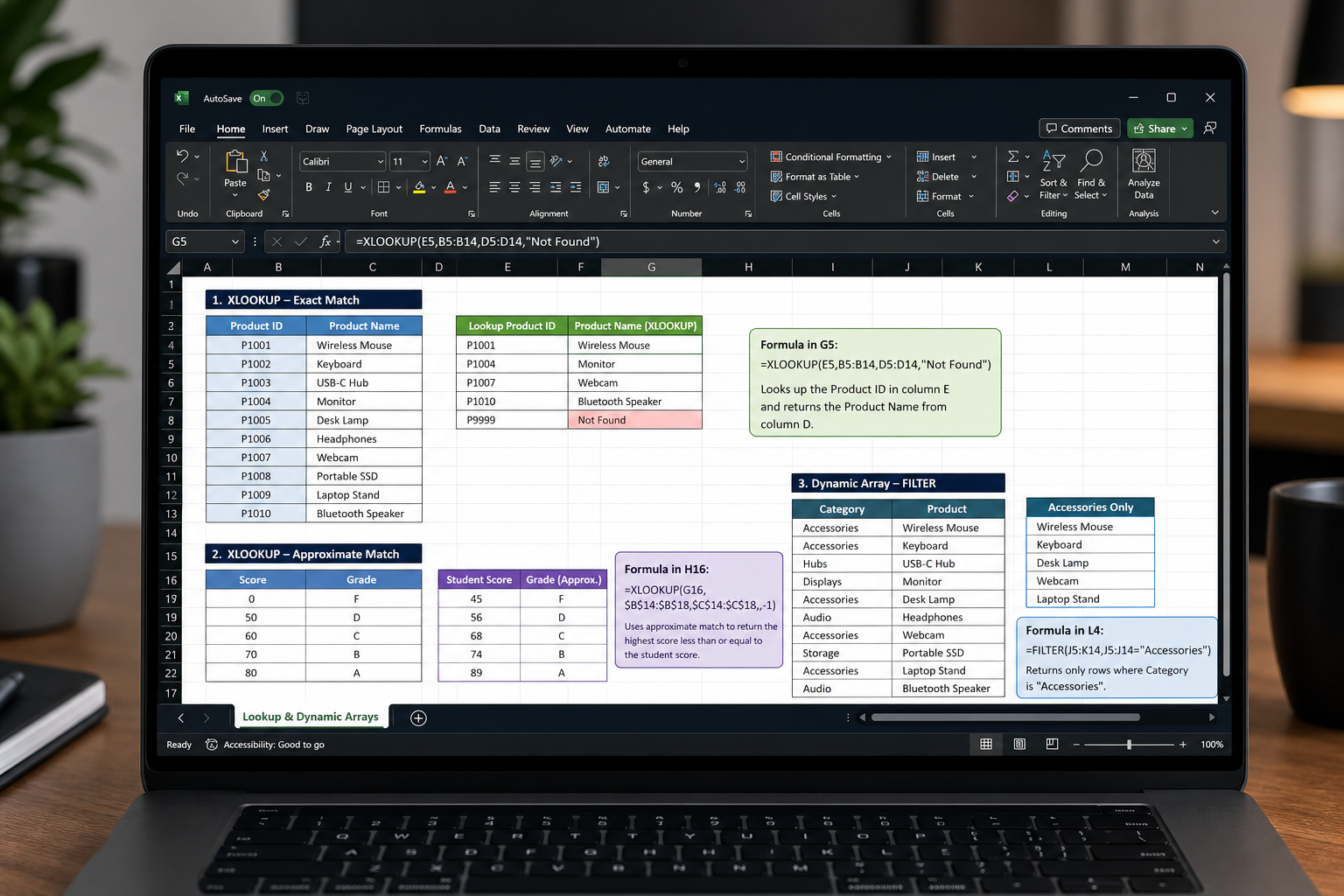
Excel power user functions are still the fastest route from raw data to a real answer in 2026 — even as Power BI dashboards and AI-assisted tools multiply around them. Knowing which formulas to reach for, and exactly when a formula beats a pivot table, separates analysts who wait for dashboards from those who build them. This guide covers the techniques that consistently deliver the highest return on time invested.

Why Excel Formulas Still Win in 2026

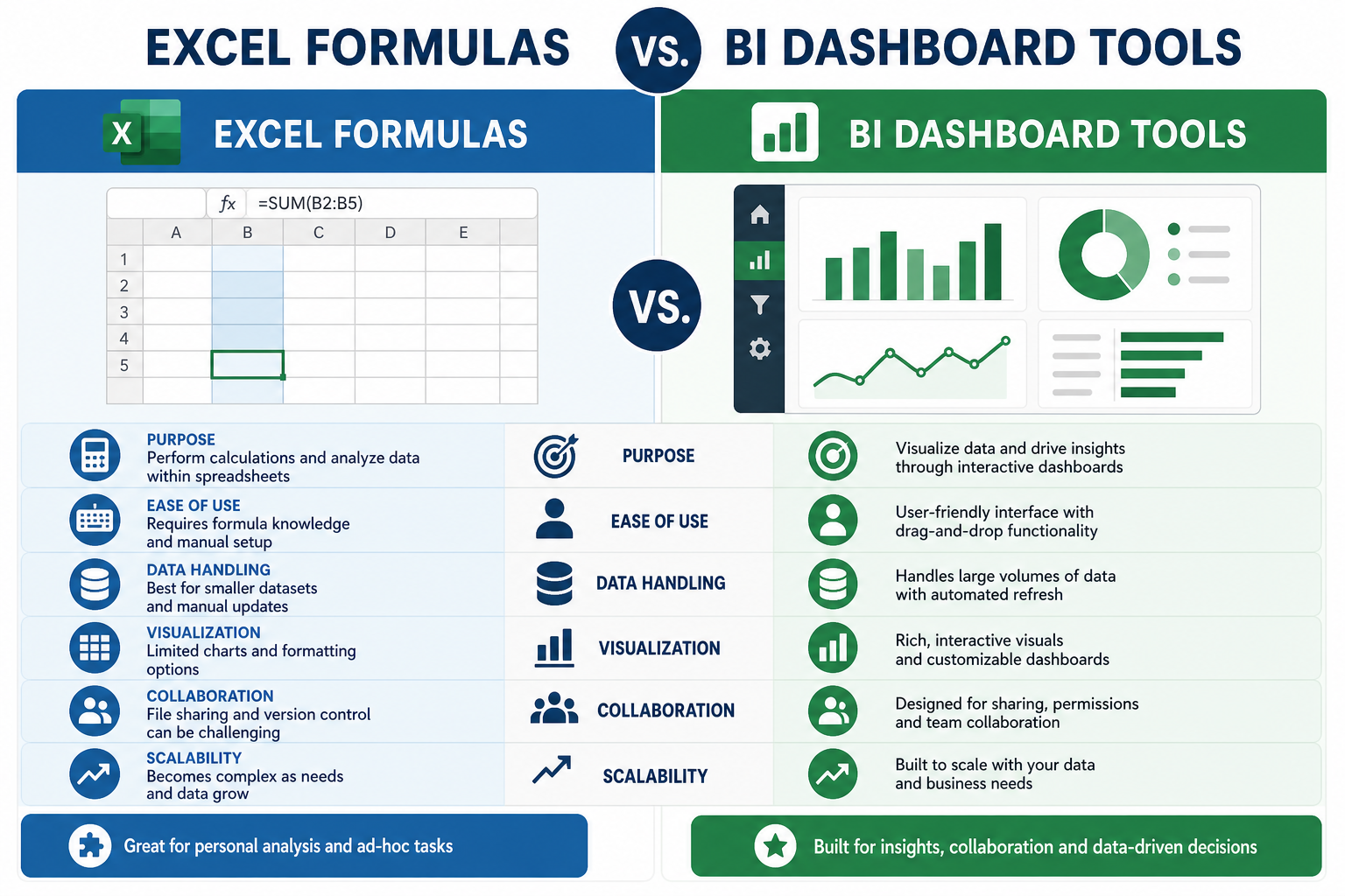
Business intelligence platforms are powerful, but they sit upstream of the decision-maker. Excel formulas sit right inside the file the stakeholder opens. When a finance director needs a quick variance check, or a project manager wants to cross-reference two lists before a morning stand-up, a well-placed Excel formula delivers the answer in seconds without a gateway to a separate BI environment. According to Microsoft, Excel is used by more than 750 million people worldwide — a user base no single BI tool comes close to matching. That ubiquity means Excel proficiency translates directly into portability: your skills work on any machine, in any organisation.

XLOOKUP Excel: The Function That Replaced a Generation of Workarounds

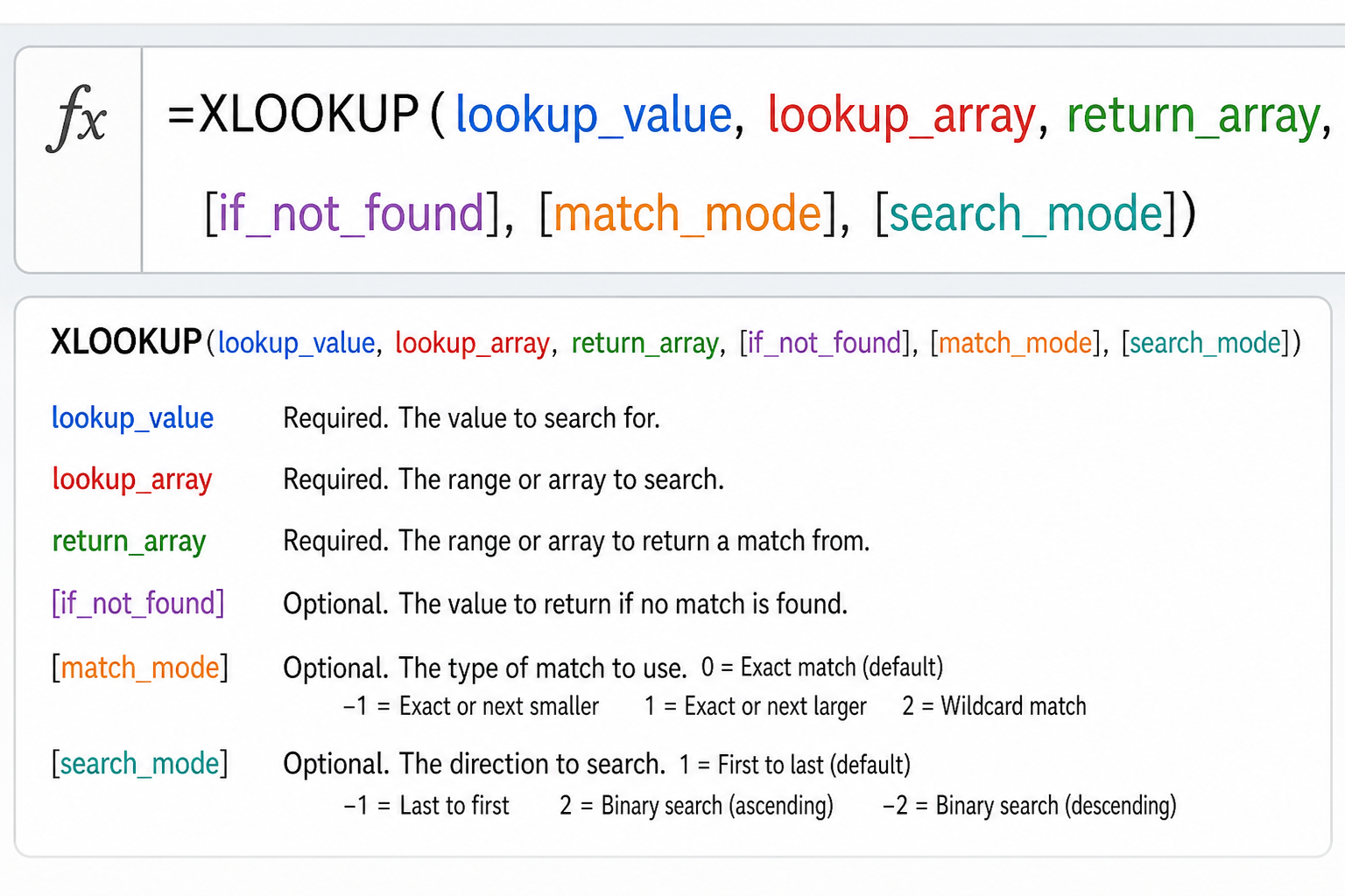
XLOOKUP Excel is the single biggest quality-of-life improvement Microsoft has shipped in years. It replaces VLOOKUP, HLOOKUP, and the classic INDEX/MATCH combination with one clean, readable function.

Basic XLOOKUP Excel Syntax

The core syntax is straightforward:

=XLOOKUP(lookup_value, lookup_array, return_array, [if_not_found], [match_mode], [search_mode])

The optional arguments are where the power lives. The if_not_found argument lets you return a custom message instead of the dreaded #N/A error — no more wrapping everything in IFERROR. The match_mode argument supports exact, approximate, and even wildcard matching in a single parameter.

XLOOKUP vs VLOOKUP: Key Differences

• Searches left or right — VLOOKUP only looks to the right; XLOOKUP has no such restriction.
• Column number is gone — you reference the return range directly, so inserting columns never breaks the formula.
• Returns an array — XLOOKUP can return multiple columns in one call, spilling results automatically.
• Reverse search — set search_mode to -1 to find the last match, not the first.
• Binary search — for very large sorted datasets, binary search mode is dramatically faster.

If you are still running VLOOKUP in 2026, switching to XLOOKUP Excel is the single highest-ROI formula upgrade available to you. For the full official reference, see the Microsoft XLOOKUP documentation.

Dynamic Arrays Excel: The Engine Behind Modern Spreadsheets

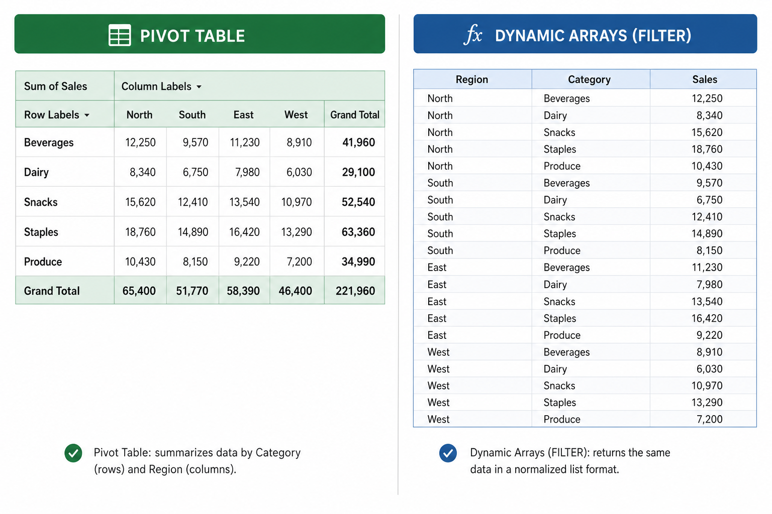
Dynamic arrays Excel introduced in 2020 fundamentally changed how results flow through a worksheet. A single formula can now spill an entire table of results into adjacent cells automatically — no Ctrl+Shift+Enter, no array wrangling.

The Core Dynamic Arrays Functions

• FILTER — returns only rows meeting one or more conditions, updating live as source data changes.
• SORT / SORTBY — sort a range by any column, including columns not in the output.
• UNIQUE — extracts a deduplicated list from a column — the instant alternative to Remove Duplicates.
• SEQUENCE — generates a grid of consecutive numbers, useful for building calendar grids, pagination logic, and more.
• CHOOSECOLS / CHOOSEROWS — pick specific columns or rows from an array without helper columns.

Chaining Dynamic Array Functions

The real productivity gain comes from nesting these together. For example, =SORT(FILTER(A2:C200, B2:B200="London")) returns a sorted, filtered subset of a large table in one cell — no helper columns, no manual refresh. Combine UNIQUE with XLOOKUP and you can build a self-updating lookup table that adapts as new categories appear in your source data.

The spill range operator (#) is the glue that connects chained formulas. Reference a spill range as A2# and any formula downstream will automatically consume however many rows the upstream formula produced.

Excel Formulas vs Pivot Tables: Choosing the Right Tool

Excel formulas outperform pivot tables in specific, predictable situations. Understanding that boundary is a core Excel power user skill.

When to Use Formulas Instead of a Pivot Table

• The output must update automatically — pivot tables require a manual Refresh; formula-driven summaries recalculate instantly.
• You need conditional aggregation across multiple criteria — SUMIFS, AVERAGEIFS, and COUNTIFS handle multi-condition aggregation in a single, auditable expression.
• The layout is fixed — if the consumer of the report needs a specific, non-negotiable table shape, a formula-built table is more reliable than a pivot that could be accidentally refreshed into a different layout.
• The workbook is shared or template-driven — pivot tables carry cache bloat and connection settings; formula ranges are lighter and more portable.
• You are feeding another formula downstream — a pivot table result cannot be directly referenced by XLOOKUP or FILTER; formula output can.

When a Pivot Table Is Still the Better Choice

Pivot tables win when a non-technical user needs to slice and drill interactively, when the dataset exceeds a few hundred thousand rows (where the Power Pivot engine helps), or when you need a quick exploratory summary before you know which questions to ask. There is no universal winner — the best Excel power users reach for both, deliberately.

High-Impact Excel Formulas Beyond XLOOKUP

XLOOKUP gets most of the attention, but several other Excel formulas deliver outsized value for daily analytical work.

LET — Name Intermediate Results

The LET function lets you assign names to intermediate calculations inside a single formula. This makes long formulas readable, eliminates repeated sub-expressions (which also speeds up recalculation), and is the closest Excel gets to a proper variable.

=LET(sales, B2:B200, costs, C2:C200, margin, (sales-costs)/sales, AVERAGE(margin))

LAMBDA — Build Your Own Excel Formulas

LAMBDA allows you to define reusable custom functions using pure Excel formula syntax — no VBA required. Once saved to the Name Manager, a LAMBDA behaves exactly like a built-in function. Combined with helper functions like MAP, REDUCE, SCAN, and MAKEARRAY, LAMBDA brings functional-programming patterns to anyone already comfortable with Excel formulas.

TEXTBEFORE / TEXTAFTER and TEXTSPLIT

Text manipulation used to mean either complex MID/FIND chains or a detour through Power Query. TEXTBEFORE, TEXTAFTER, and TEXTSPLIT handle the most common text-parsing tasks — splitting on a delimiter, extracting everything before a separator — in one readable function. For data-cleaning workflows that used to take five minutes, these functions take five seconds.

BYROW and BYCOL

These helper functions apply a LAMBDA expression to each row or column of a range and return a single-column or single-row result. They replace the pattern of dragging a helper column formula down an entire dataset and then referencing that helper — the calculation stays inside one expression.

Practical Workflows That Combine These Excel Formulas

The techniques above compound when combined. Here are three practical patterns that senior analysts use regularly.

Self-Updating Report Tables

Build the master data table as a structured Excel Table (Ctrl+T). Then use FILTER to extract the relevant subset, SORT to order it, and XLOOKUP to pull in reference data from another sheet. Add a slicer-equivalent using a dropdown validation list tied to a UNIQUE formula, and the report updates the moment new rows land in the source table — no pivot refresh, no macro.

Error-Free Multi-Sheet Lookups

Classic VLOOKUP across multiple sheets required INDIRECT or repetitive IFERROR nesting. With dynamic arrays Excel and XLOOKUP, you can wrap multiple sheet references in a single expression and return the first non-empty match cleanly, with a custom fallback message if nothing is found across any of the sheets.

Data Validation With FILTER and UNIQUE

Rather than hard-coding dropdown lists in Data Validation, reference a UNIQUE formula output as the source. As new values appear in the source column, the dropdown updates automatically — a small change that eliminates a common maintenance headache in template-based workbooks.

Getting the Right Version of Excel

Most of the functions covered here — XLOOKUP, FILTER, SORT, UNIQUE, LET, LAMBDA, TEXTSPLIT, BYROW — are available in Excel for Microsoft 365 and Excel 2024 for Windows. If you are running an older perpetual version, XLOOKUP and dynamic arrays will not be available. Upgrading to a current perpetual licence is the fastest path to unlocking all of them without a subscription. You can also get the full Office suite including Excel through an Office 2021 licence, which includes XLOOKUP and the core dynamic array functions.

Choosing a perpetual licence over a recurring subscription makes long-term financial sense for individuals and small teams who do not need the very latest cloud-first features — the core Excel power user functions you will use every day are all present in the perpetual builds.

FAQ

Is XLOOKUP available in Excel 2019?

No. XLOOKUP was introduced for Microsoft 365 subscribers in 2019 and is included in Excel 2021 and Excel 2024 perpetual licences. It is not available in Excel 2019 or earlier perpetual versions. If you need XLOOKUP, upgrading to at least Office 2021 is the straightforward solution.

Do dynamic arrays Excel functions slow down large workbooks?

They can, but the impact is usually modest for datasets under 100,000 rows. The main causes of slowdown are volatile functions (RAND, NOW, INDIRECT) inside spill ranges, or very deeply nested dynamic array chains. Using LET to avoid recalculating the same sub-expression multiple times is the most effective mitigation for complex formula sets.

When should I use XLOOKUP instead of INDEX/MATCH?

For most use cases in 2026, XLOOKUP is the better choice — it is shorter, more readable, and handles left-side lookups and multiple return columns natively. INDEX/MATCH still has a role in very large datasets where binary search performance matters and in workbooks that must be backward-compatible with pre-2021 Excel versions.

Can LAMBDA functions replace VBA macros?

For calculation logic, yes — LAMBDA can replicate a large proportion of what simple VBA functions do, without requiring the Trust Center settings that macros need. However, VBA is still needed for anything that interacts with the user interface, triggers on events, or calls external APIs. Think of LAMBDA as covering formula automation; VBA for everything else.

What is the difference between FILTER and a pivot table filter?

A pivot table filter hides rows from a pre-aggregated view and requires a manual refresh to pick up new source data. The FILTER function returns a live, formula-driven subset of the source range that recalculates automatically and can be chained with other dynamic array functions. FILTER output can also be directly referenced by other formulas; pivot table filtered results cannot.