
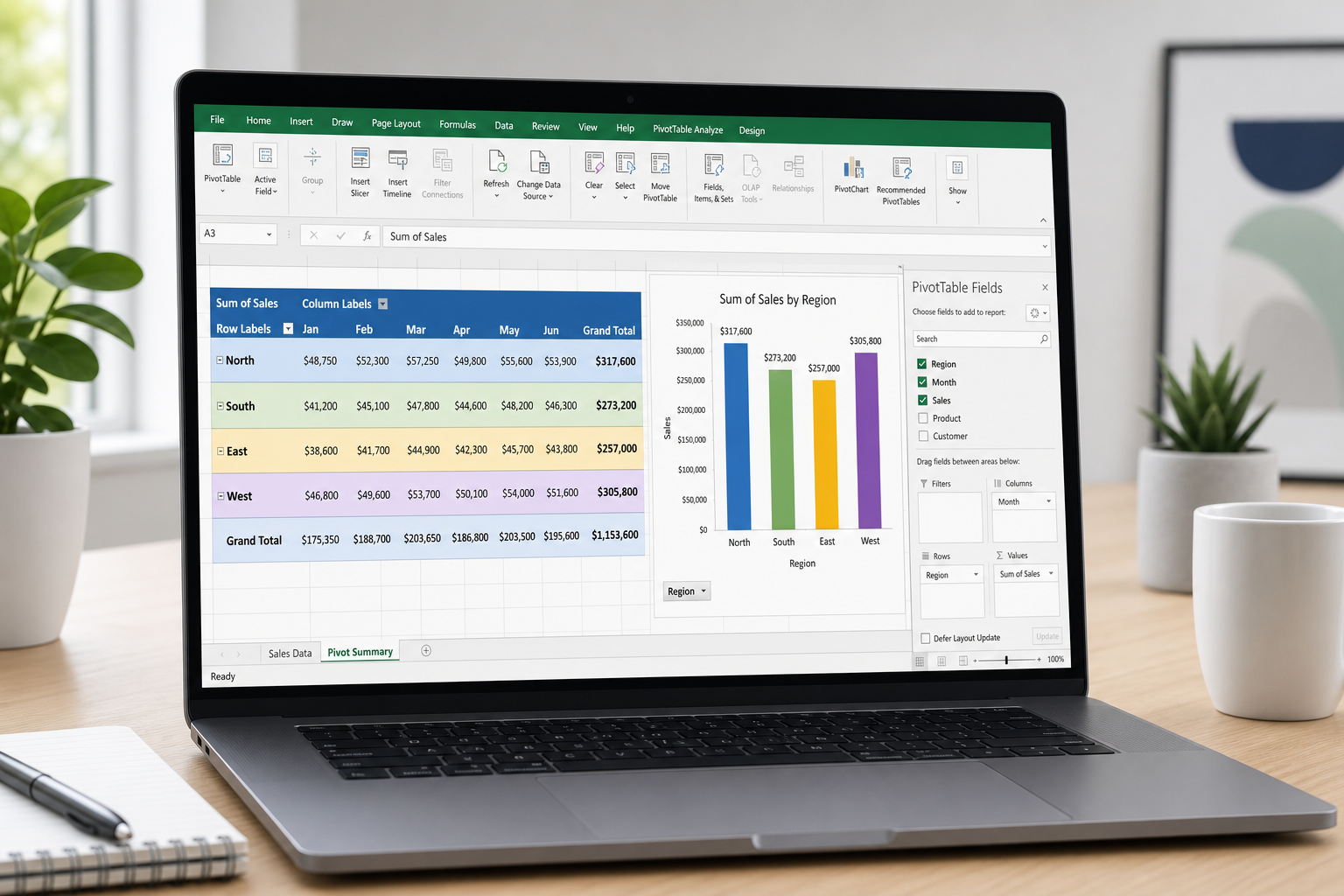
Excel pivot tables let you turn hundreds (or thousands) of rows of raw data into a clean summary table in a few clicks, without writing a single formula. If you’ve ever scrolled through a spreadsheet trying to manually add up totals by category, a pivot table does that work for you instantly, and lets you rearrange the summary just by dragging fields around.
This guide walks through building your first Excel pivot table, grouping data so it actually makes sense, and the mistakes that trip up almost every beginner.
What Are Excel Pivot Tables and Why Do You Need One?
An Excel pivot table is a tool that automatically summarizes, counts, and calculates data from a larger table without changing the original data. It’s the fastest way to answer questions like “which product sold the most last quarter” or “how many hours did each employee log” without writing a single SUMIF or COUNTIF formula.
Think of raw spreadsheet data as a pile of receipts — useful, but hard to read at a glance. A pivot tables sorts that pile into labeled stacks: totals by region, by month, by category, or by any combination you choose. For students compiling survey results or small business owners reviewing sales, this is usually the single most useful feature in Excel.
Preparing Your Spreadsheet Before Building Excel Pivot Tables
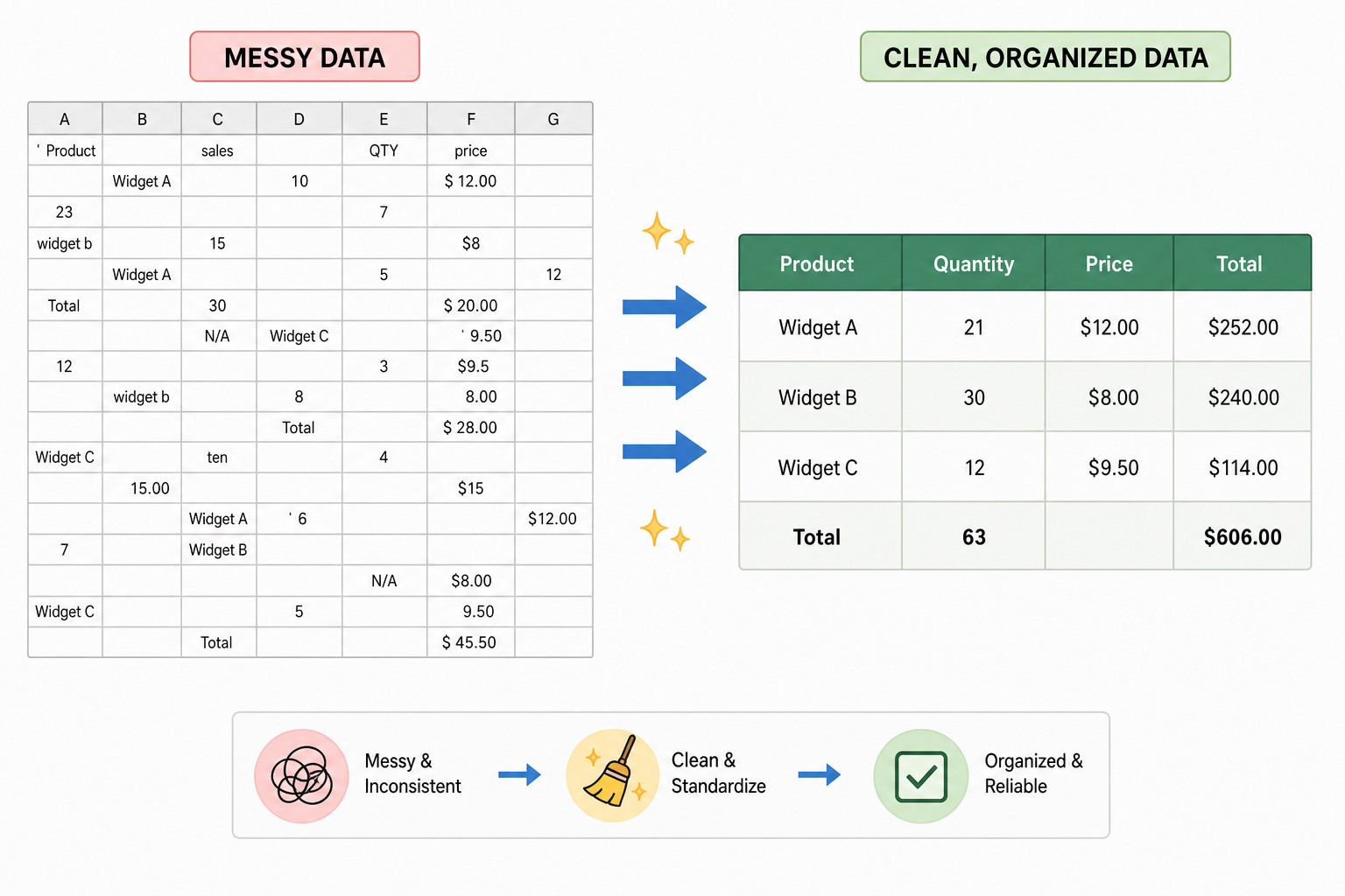
Excel pivot tables only work well when the source data is structured correctly. Before inserting one, check these basics:
-
Every column has a single, unique header in the first row — no blank or merged header cells.
-
Each row represents one complete record (one sale, one student, one transaction).
-
There are no fully blank rows or columns inside the data range.
-
Numbers are formatted as numbers, and dates as dates — not as text.
-
Each column holds one type of data consistently (don’t mix text and numbers in the same column).
If your spreadsheet fails any of these checks, fix it first. Pivot tables built on messy source data will produce misleading summaries, and troubleshooting a bad pivot table is much slower than cleaning the data upfront.
How to Build Your First Pivot Tables in Minutes
You can build a working Excel pivot table in under five minutes once your data is clean. The official Microsoft Excel documentation covers every platform, but the core steps are the same everywhere.
Step 1: Select the Data for Your Pivot Table
Click anywhere inside your data range, or select it manually if it includes blank rows you want to exclude. Excel usually detects the full range automatically when you start the next step, so you rarely need to select every cell by hand.
Step 2: Insert the Pivot Table
Go to Insert > PivotTable. Excel will suggest a range and ask whether you want the pivot table on a new worksheet or the existing one. Choosing a new worksheet keeps your source data untouched and the summary easy to find.
Step 3: Arrange Fields in the Pivot Table Layout
A field list appears on the right with four boxes: Filters, Columns, Rows, and Values. Drag the field you want to group by (like “Region” or “Month”) into Rows, and drag a numeric field (like “Sales”) into Values. Excel will automatically sum the numbers for each group. That’s it — you have a working pivot table.
Grouping Data in Excel Pivot Tables
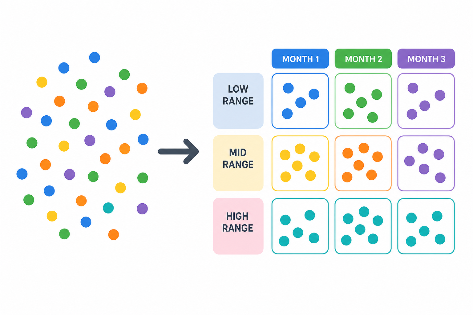
Grouping is what turns a long list of individual entries into a readable summary, and it’s one of the most underused features in Excel pivot tables. Instead of seeing every single date or number, you group related values together into buckets.
Grouping Dates Into Months or Quarters
Right-click any date in the Rows area of the pivot table and select Group. Excel lets you group by days, months, quarters, or years — or a combination, such as years and months together. This is especially useful for turning a year of daily transaction data into a clean monthly trend.
Grouping Numbers Into Ranges
For numeric fields like age, price, or score, right-click a value and choose Group again. You can set a starting number, an ending number, and an interval (for example, grouping ages into 10-year bands). This converts a scattered list of individual numbers into a handful of meaningful ranges.
Grouping doesn’t alter your source data at all — it only changes how the pivot table displays it, so you can experiment freely and regroup at any time.
Common Excel Pivot Table Mistakes (and How to Avoid Them)
Most pivot table problems come from the source data, not the pivot table itself. These are the mistakes beginners run into most often:
-
Leaving blank rows inside the data range. Excel stops reading data at the first fully blank row, silently cutting off everything below it.
-
Using merged cells in headers. Merged header cells confuse the field list and can make fields disappear entirely.
-
Mixing text and numbers in one column. A column with “1,200” as text and 1200 as a number will be summed incorrectly or not at all.
-
Forgetting to refresh after adding new rows. New data added below the original range won’t appear until you manually refresh.
-
Not naming the data as a Table. Converting your range into a named Table (Ctrl+T) before building Excel pivot tables means new rows are picked up automatically on refresh.
If a pivot table looks wrong, check the source data for one of these issues first — it’s almost always the cause.
Keeping Your Pivot Table Data Up to Date
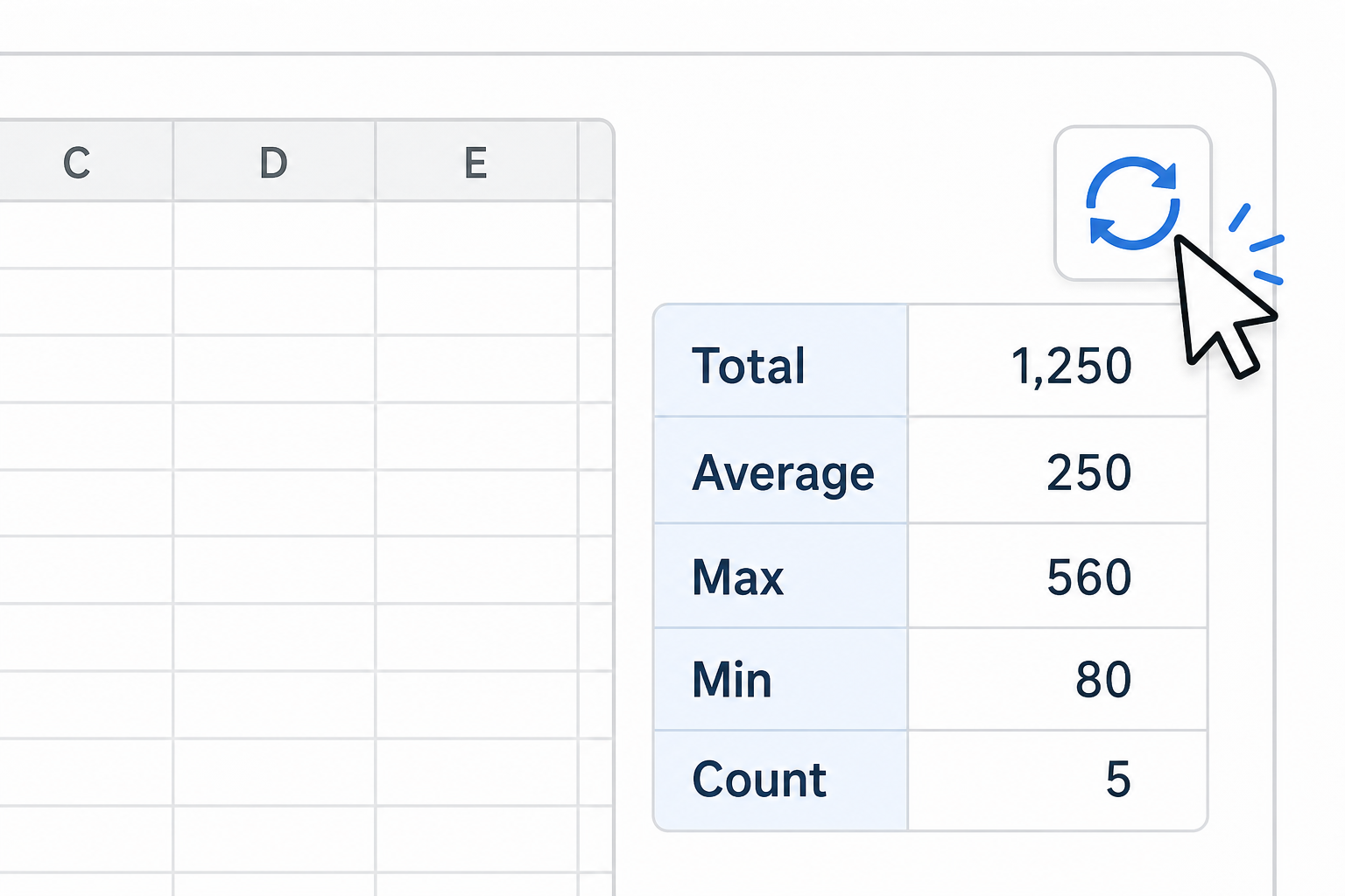
A pivot table does not update automatically when the source data changes — you have to tell it to refresh. Right-click anywhere inside the pivot table and choose Refresh, or use the Refresh button on the PivotTable Analyze tab. If you’ve added new rows beyond the original range, you may also need to update the data source range under PivotTable Analyze > Change Data Source.
For spreadsheets that get new data regularly — weekly sales logs, attendance sheets, survey responses — it’s worth converting the source range into a proper Excel Table first. Tables expand automatically, so Excel pivot tables built on them pick up new rows with a single refresh instead of a manual range edit.
Where to Get Excel for Building Pivot Tables
Pivot tables are available in every modern version of Excel, including the standalone, one-time-purchase editions that don’t require a subscription. If you’re setting up a new PC or replacing an old license, Excel 2024 for Windows is available at Top Key Shop for €42.90 with an official activation key and download link.
Students and home users who also need Word, PowerPoint, and Outlook alongside Excel may find a full suite more practical — the Office 2021 Home and Student for Windows license includes Excel with the other core apps in a single one-time purchase.
Once pivot tables feel comfortable, there’s a lot more Excel can do for repetitive reporting and analysis — our rundown of Excel power user functions covers lookups and dynamic arrays that pair well with pivot tables for more advanced summaries.
FAQ
What is a pivot table used for in Excel?
A pivot table summarizes large sets of data into totals, counts, or averages grouped by the categories you choose, without needing formulas. It’s commonly used for sales reports, survey analysis, budget tracking, and any situation where you need a quick summary from a long list of raw entries.
Do I need to know formulas to use Excel pivot tables?
No. Excel pivot tables are built with drag-and-drop fields rather than formulas, which is exactly why they’re a popular starting point for beginners. Excel automatically handles the sums, counts, and averages once you place fields into the Values area.
Why is my pivot table showing blank or wrong values?
This usually comes from a problem in the source data rather than the pivot table itself — commonly blank rows inside the data range, numbers stored as text, or merged header cells. Fixing the source data and refreshing the pivot table almost always resolves it.
Can I create a pivot table from multiple sheets?
Yes, using Excel’s Data Model or Power Pivot feature, you can combine tables from multiple sheets or even multiple files into one pivot table. For most everyday tasks, though, consolidating the data onto one sheet first is simpler and less error-prone.
How do I update a pivot table after adding new data?
Right-click inside the pivot table and select Refresh, or press Alt+F5. If the new rows fall outside the original data range, update the range under PivotTable Analyze > Change Data Source, or convert your source data into an Excel Table first so it expands automatically.
Is a pivot table the same as a pivot chart?
No — a pivot chart is a visual chart built from a pivot table’s summarized data. You typically build the pivot table first to get the numbers right, then insert a pivot chart from it to present the same summary visually.
